QuantPy: Portfolio Optimization

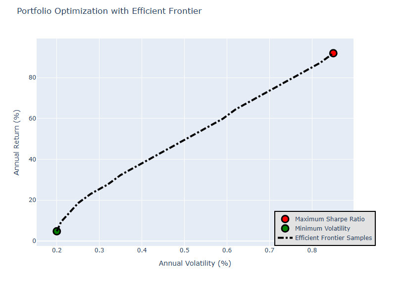
QuantPy is a Python library and research framework I built to apply quantitative finance algorithms to real equity portfolios. Given a set of ticker symbols, it pulls historical price data from Yahoo Finance, constructs the statistical model of the asset universe, and then runs a suite of numerical optimization algorithms to find the allocation that best balances return and risk. The end result is an interactive efficient frontier plot that surfaces the maximum Sharpe ratio portfolio and the minimum variance portfolio alongside any target-return allocation the user specifies.

What It Does

You pass QuantPy any list of equity tickers (individual stocks, ETFs, sector funds, currencies) and it:

Fetches daily closing prices via yfinance and forward-fills missing sessions
Computes daily log-returns and annualizes them to APY per asset
Builds the mean-return vector and full covariance matrix across all assets
Runs three constrained optimizations to find optimal weight vectors
Traces 20 points along the efficient frontier between the minimum-variance and maximum-Sharpe portfolios
Renders an interactive Plotly chart of the frontier with the two landmark portfolios highlighted

Algorithms Implemented

Covariance Matrix & Return Statistics

The foundation of Modern Portfolio Theory is the statistical relationship between assets. QuantPy computes the daily percentage-change return series for every ticker and then builds the full N×N covariance matrix Σ using Pandas:

self.returns = self.allEquities.pct_change()[1:]
self.meanReturns = self.returns.mean()
self.covMatrix = self.returns.cov()

Portfolio variance for a weight vector w is then the bilinear form σ² = wᵀ Σ w, evaluated via NumPy dot products.

Sharpe Ratio Maximization

The Sharpe ratio measures return per unit of risk: S = (Rp - Rf) / σp. To find the allocation that maximizes it, QuantPy minimizes the negative Sharpe ratio subject to the constraint that weights sum to 1, using SciPy's Sequential Least Squares Quadratic Programming (SLSQP) solver:

result = sc.minimize(
    self.negativeSharpeRatio,
    numAssets * [1. / numAssets],   # equal-weight starting point
    args=(riskFreeRate),
    method='SLSQP',
    bounds=tuple((0, 1) for _ in range(numAssets)),
    constraints={'type': 'eq', 'fun': lambda x: sum(x) - 1}
)

The cumulative return over the full date range is used in the objective rather than the arithmetic mean, making the optimizer sensitive to compounding and drawdown path.

Minimum Variance Portfolio

A separate optimization finds the allocation with the lowest absolute volatility, regardless of return. This is the leftmost point on the efficient frontier: the portfolio with the least possible risk.

result = sc.minimize(
    self.portfolioVariance,
    numAssets * [1. / numAssets],
    method='SLSQP',
    bounds=bounds,
    constraints={'type': 'eq', 'fun': lambda x: sum(x) - 1}
)

Target-Return Optimization (Efficient Frontier Tracing)

For any target return R*, QuantPy can find the allocation with the minimum variance that hits exactly that return. This adds a second equality constraint to the SLSQP problem:

constraints = (
    {'type': 'eq', 'fun': lambda x: self.portfolioReturn(x).iloc[-1] - returnTarget},
    {'type': 'eq', 'fun': lambda x: sum(x) - 1}
)

By sweeping returnTarget across 20 linearly spaced values from the minimum-variance return to the maximum-Sharpe return, QuantPy traces the full efficient frontier curve.

Closed-Form Analytical Weights (Two-Fund Separation)

In addition to the numerical optimizer, QuantPy implements the closed-form analytical solution from Markowitz theory. Any efficient portfolio can be expressed as a linear combination of two "fund" portfolios: the characteristic (minimum variance) portfolio w_c and the tangency (Sharpe-optimal) portfolio w_q, via the Two-Fund Separation Theorem:

w = (fq - fp) * wc + (fp - fc) * wq

where f_c and f_q are the returns of each fund and f_p is the target return. Each fund weight is computed analytically from the inverse covariance matrix:

iV = matrix(inv(self.cov()))
w = array(iV * e / (e.T * iV * e)).flatten()

This gives the exact solution without requiring iterative optimization for points along the frontier.

Portfolio Performance & Cumulative Returns

Portfolio daily returns are computed as the weighted sum of individual asset returns. Cumulative return compounds them via cumprod:

weightedReturns = self.returns * weights
dailyPortfolioReturns = weightedReturns.sum(axis=1)
cumulativeReturns = (dailyPortfolioReturns + 1).cumprod() - 1

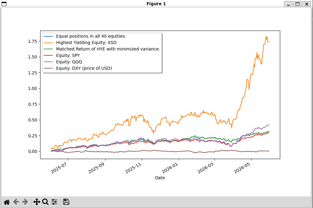
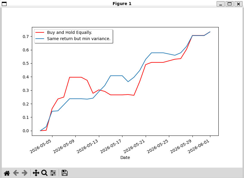
This lets the library compare any allocation strategy (equal-weight, max-Sharpe, min-variance, single-ticker) on a normalized cumulative basis over the same time window.

Example Output

Running the optimizer on a diversified watchlist of 40+ tickers (technology, energy, commodities, covered-call ETFs, nuclear, biotech, and consumer staples) produces a Plotly chart showing:

The efficient frontier curve (risk vs. return tradeoff across all feasible allocations)
The maximum Sharpe ratio portfolio (the tangent point on the capital market line)
The minimum volatility portfolio (the leftmost point on the frontier)
Overlaid cumulative return traces comparing equal-weight, Sharpe-optimal, and individual benchmark tickers (SPY, QQQ, DXY)

Tech Stack

Python · NumPy · Pandas · SciPy (SLSQP) · yfinance · Plotly · Matplotlib · Modern Portfolio Theory · Markowitz Efficient Frontier · Sharpe Ratio Optimization · Two-Fund Separation Theorem · Covariance Matrix · Constrained Nonlinear Optimization

Jake Mitchell